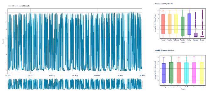
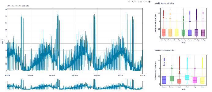
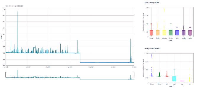
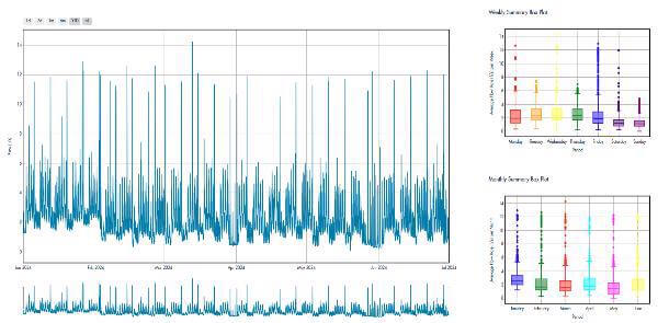
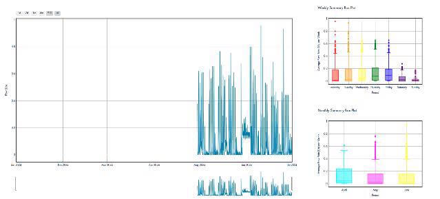
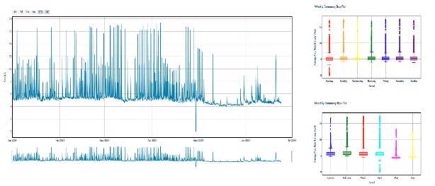
Figure 1: A few representative time series and their weekly and monthly distribution showcasing the types of time series pattern of CLU data.
The value of time series analysis lies in its ability to uncover underlying patterns and trends within temporal data, enabling us to predict and forecast future values accurately. Furthermore, time series analysis plays a critical role in imputing missing data, thereby preserving the integrity and usability of the dataset.
In the context of time series analysis, prediction or forecasting involves estimating future values 𝒀𝒕+𝒌 of the series based on its past values 𝒀𝒕 , 𝒀𝒕−𝟏, … , 𝒀𝒕−𝒏. Here, 𝒕 represent the current time, and 𝒌 is the number of future time steps we aim to predict. On the other hand, imputation refers to filling in missing values, 𝒀𝒕𝒊 within the existing dataset, where 𝒕𝒊 represents the time points with missing data. By reconstructing a complete dataset, imputation ensures continuity of the series.
Consider the animation below as a demonstration of prediction, imputation, and forecasting in action. This visual illustrates how time series analysis can be applied to effectively predict future values and handle missing data.
The quest to develop accurate prediction and forecasting models is driven by the immense benefits they offer. We are getting access to more data than ever before, and the availability of advanced computing power and tools have revolutionized time series prediction. However, real-world time series data is also complex and messy. Our aim is to develop an approach or a combination of approaches that can take care of prediction, forecasting and imputation relevant to the various types of patterns, complexity, and state of the CLU data.
Traditional time series analysis methods have been foundational in understanding and forecasting time series data. They are effective for making short-term forecasts and handling missing data. However, these methods may not fully capture complex patterns in data. We list out some of these methods below.
MA is known to be simple, yet powerful technique used to forecast time series data. The Simple Moving Average (SMA)
where 𝑌_𝑡 is the value at time 𝑡, 𝑛 is the number of data points in the moving window, calculates the average of the last 𝑛 data points. This helps to smooth the data by averaging out short-term fluctuations, making it easier to see long-term trends.
Given a simulated “True” data, we present the animation below to demonstrate SMA using three different windows and how each fare in predicting the True data.
Exponential Smoothing assigns decreasing weights (importance) to older observations, giving more importance to recent data. It includes Single Exponential Smoothing (SES), Double Exponential Smoothing (DES) and Triple Exponential Smoothing (TES). It is known to be suitable for time series data with a level, trend, and seasonal components.
Where 𝑆𝑡 is the smoothed value at time 𝑡, 𝛼 is the smoothing factor, and 0 < 𝛼 < 1. SES updates the smoothed value 𝑆𝑡 by combining the actual value 𝑌𝑡 and the previous smoothed value 𝑆𝑡−1 . The smoothing factor determines how much importance is given to the recent observation compared to the past smoothed values.
Where 𝑇𝑡 is the trend estimate at time t, 𝛾 is the trend smoothing factor. DES is used for time series with trends. It calculates both the smoothed value and trend separately. The smoothed value considers the current observation and the previous smoothed value plus the trend. The trend is updated based on the change in smoothed value.
Where 𝐶𝑡 is the seasonal component, 𝐿 is the length of the seasonal cycle, and 𝛽 and 𝛾 are smoothing factors for trend and seasonality. TES, otherwise known as Holt-Winters methods, account for seasonality in addition to trends. It uses three equations to update the smoothed value, trend, and seasonal components, capturing more complex patterns in data.
Spline interpolation fits a curve through the known data points, making it useful for interpolating missing values in time series data. Spline interpolations make use of polynomial functions. For instance, a linear spline uses a linear function to connect each data point with a straight line, a cubic spline uses a smoother piecewise cubic function that passes through the known data points.
The Kalman Filter is a probabilistic approach used to estimate the state of a dynamic system from a series of noisy measurements. It is an iterative process using a series of inputs to produce estimates of unknown variables. It is effective in smoothing time series data and filling missing values by considering statistical noise and inaccuracies. The Kalman Filter operates in two steps:
- Predict: Project the current state and error covariance forward to obtain the ‘a priori’ estimate for the next time step.
- Update: Incorporate new measurements to obtain the ‘a posteriori’ estimate.
Machine learning and deep learning techniques offer advanced capabilities for time series predictions and forecasting. These techniques can capture patterns and relationships in the data, making them suitable for long-term forecasts and more intricate time series. Machine learning and deep learning in the context of time series involve using algorithms that can learn from and make predictions concerning sequential data. Unlike traditional statistical methods, which often rely on the predefined models and assumptions (equations and its parameters), machine learning techniques adaptively learn patterns from the data itself. This flexibility allows machine learning models to capture nonlinear relationships and interactions within the data, making them powerful tools for time series forecasting.
We present some of the most prominent machine learning and deep learning techniques being used across different domains.
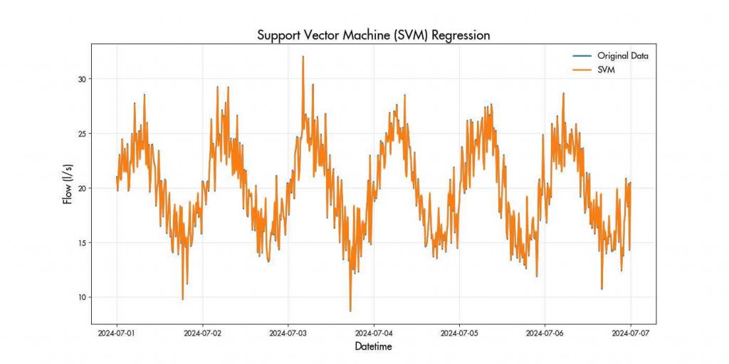
SVM is a type of supervised learning method that is known to be effective in capturing non-linear relationships. For time series, SVM Regression aims to fit the data and predict future values. For a set of training data points (𝑥𝑖 , 𝑦𝑖 ) where 𝑥𝑖 represents the input features and 𝑦𝑖 represents the target values.
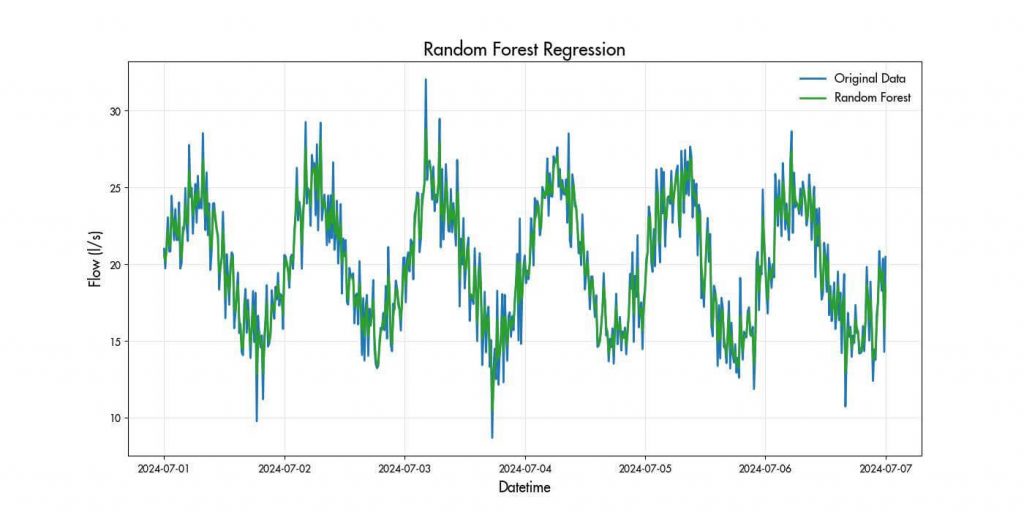
Random Forests use multiple decision trees to make predictions, averaging the results to improve accuracy. They are very effective for time series forecasting due to their ability to capture various patterns and handle large datasets.
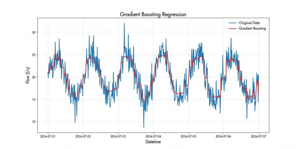
GBM builds models sequentially, each new model aiming to reduce errors from previous ones. This approach makes GBMs highly accurate and suitable for time series forecasting where capturing patterns is essential.
Deep Learning, a subset of machine learning, involves neural networks with multiple layers that can automatically learn feature representations from data. Deep learning models are particularly effective at capturing complex temporal dependencies and patterns that may be difficult to identify with traditional methods.
LSTM networks are a type of recurrent neural network (RNN) that are wellsuited for time series forecasting because they can learn long-term dependencies and remember information for extended periods. The key components of LSTM include:
- The “Cell State” which is essentially the memory of a network. It is designed to carry information across sequences, helping network remember context over many times steps.
- The “Forget Gate” that determines what information should be discarded in the cell state.
- The “Input Gate” that decides which new information should be stored in the cell state.
- The “Update Stage” where the cell state is computed by combining the old cell state and new candidate values.
- The “Output Gate” that determine the output based on the cell state.
These components allow LSTMs to learn complex patterns in time series data.
In this blog, we presented various methods for time series analysis, compared their effectiveness, discussed some of the underlying mathematics, and provided animations demonstrating the implementation of each of the methods. We have reviewed Moving Averages, Exponential Smoothing, Spline Interpolation, and Kalman Filter, which are foundational methods employed for prediction, imputation and forecasting of time series with varying types and behaviour. We also took a look at Support Vector Machines, Random Forests, Gradient Boosting Machines, and LSTM. These methods provide advanced capabilities for capturing complex patterns and improving the accuracy of predictions.
The limitations of both traditional and modern methods highlights the need for a hybrid approach. A hybrid method combines the strengths of multiple approaches for better imputation and improves the accuracy and robustness of predictions. The varying types of patterns and behaviour of CLU data warrants a combination of approaches that will leverage their collective strengths and adapt to different data characteristics.
In my next blog, we will dive deeper into the hybrid approach, building the hybrid models and exploring comprehensive comparisons between traditional and modern methods with examples and case studies.