CLU Hybrid – A Multi Method Approach to Imputation and Forecasting

In our previous blog, we discussed the importance of time series data across various domains, from finance to the water industry, and highlighted the challenges of missing data and accurate forecasting. We reviewed both traditional and modern time series analysis techniques and recognized that no single method works best in every scenario. Addressing these challenges effectively requires a blend of these methods to leverage their strengths.

In this blog, we present our implementation of CLU Hybrid, a multi method approach tailored for Continuously Logged Users (CLU) time series data. CLU data, which captures large water consumption at 15-minute interval, exhibits distinctive characteristics—including seasonal, cyclical, and persistent trends—along with irregular fluctuations and data integrity challenges. Understanding these characteristics is crucial to the accurate imputation of data gaps and further forecasting.

In the absence of actual CLU data, our strategy focuses on accurately estimating missing values—referred to as CLU Estimated—to enhance the reliability of subsequent DMA analysis and forecasts.   

A result of our CLU Hybrid implementation is shown in Figure 1. 

CLU Hybrid involves systematically applying various imputation techniques, evaluating their performance, and selecting the optimal one based on performance (statistical) metrics. This ensures that missing CLU values are filled in the most datacentric manner – preserving the underlying data pattern and enhancing the accuracy of prediction and forecasting. 

Our implementation includes a well-orchestrated workflow that includes data extraction, gap analysis, imputation, evaluation, fallback and forecasting. Figure 2 provides a map of the CLU Hybrid implementation, which we will discuss in order below. 

The workflow begins with raw CLU data extracted from sources, then pre-processed into a format that would lend itself to analysis. For instance, datetime data would need to be transformed into datetime objects, adjusted to account for local time zone (or other time zones), and datetime data might also need reindexing to ensure consistency in time stamps. 

A comprehensive gap analysis identifies the locations and durations of missing values. Based on gap duration, different imputation methods are recommended. 

Table 1: Gap Analysis and Corresponding Imputation Methods

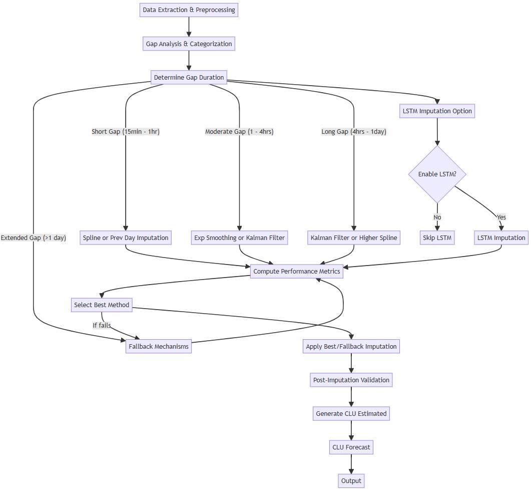
The core of the approach lies in the implementation of multiple imputation algorithms, each suited to handle different types of missing data gaps and data characteristics identified during the gap analysis. The following methods are integral to this strategy:

• Kalman Filter Imputation: 

This method treats the time series as a dynamic system, starting out with initial estimates, and then continuously updating these estimates as new information becomes available, allowing us to capture underlying patterns and trends over time. The Kalman Filter begins by initially filling missing values using forward padding to provide a baseline. It is then initialized with parameters derived from the CLU data’s mean and variance. Through an iterative optimization technique called Expectation-Maximization (EM) steps, the filter refines its estimates, smoothing out noise and predicting missing values. Post-imputation validation is in place to make sure that no residual anomalies or unrealistic values persist. 

• Exponential Smoothing Imputation

This approach is a forecasting technique that applies weighted averages of past observations, with weights decreasing exponentially over time. This method excels in capturing trends and seasonal patterns within the data, making it suitable for imputing missing values in datasets exhibiting such characteristics. After an initial interpolation to address minor gaps, the Exponential Smoothing model is configured with additive components for trend and seasonality. In this additive framework, the trend components assume linear progression over time, adding a constant increment while the seasonal component captures recurring fluctuations by adding a fixed seasonal effect to the overall level. By fitting this model to the data, it forecasts missing values as the sum of these additive components, resulting in smooth, datacentric imputation that effectively reflect underlying temporal patterns. 

• Spline Interpolation Imputation

Spline Interpolation employs mathematical functions to create a smooth curve that passes through known data points. Depending on the degree of the spline—cubic or linear—this method can adapt to varying data characteristics. The process begins with interpolating small gaps to stabilize the data, then selecting an appropriate spline degree, based on the underlying trend. The chosen spline is fitted to the non-missing data points and subsequently used to estimate the missing values. Validation steps are in place to make sure that the imputed data maintains integrity without introducing unrealistic fluctuations.

• Previous Day Imputation 

We leverage strong daily patterns by filling in missing values with data from the same time point on the previous day. This method is particularly effective for datasets with strong daily seasonality – when the underlying data is influenced by daily cycles, such as human activity, business hours, or processes that adhere to the day-night cycle. For this imputation, we first identify the start of each missing interval, we then shift the previous data forward or backwards by one day to fill in the gaps. Post-imputation validation ensures that no new, missing or infinite values are introduced, preserving the dataset’s integrity.

• LSTM–Based Imputation

We integrate a Long Short-Term Memory (LSTM) neural network into our imputation workflow to capture complex temporal dependencies and patterns that other methods might miss. LSTM is especially useful for time series data because it can learn long-term dependencies. A comprehensive discussion on LSTM could easily warrant its own post but, for now, it is important to note that while LSTM-based imputation can capture non-linear patterns and improve imputation quality, it is computationally and time expensive to implement. Therefore, we disable the LSTM module when volume of data makes LSTM training and imputation impractical. 

With multiple imputation methods at hand, determining the most effective one for a CLU dataset is at the heart of the strategy. The selection process is grounded in the evaluation of performance metrics that quantitatively assess each method’s efficacy. 

• Mean Squared Error (MSE): Measures the average squared difference between the imputed and actual values, capturing the magnitude of errors. 
• Mean Absolute Error (MAE): Calculates the average absolute difference, providing a straightforward measure of accuracy. 
• Mean Absolute Percentage Error (MAPE): Expresses errors as a percentage, facilitating comparisons across different scales. 
• R-squared (R²): Indicates the proportion of variance in the dependent variable explained by the imputed values, reflecting the method’s explanatory power. 

Each imputation method is applied to the dataset, and the resulting imputations are compared against the observed (non-missing) data using the identified metrics. By aggregating these metrics into a composite score, the method with the lowest combined score is identified as the best-performing imputation technique. This objective evaluation makes sure that the selected method not only fills in the missing values but does so with minimal error and staying close to the underlying data characteristic. 

Despite meticulous selection, certain datasets may pose challenges where all primary imputation methods fail—be it due to unforeseen data patterns, excessive “missingness”, or computational and algorithmic constraints. To safeguard against such scenarios, a fallback mechanism is in place. 

The fallback strategy involves sequentially applying alternative imputation methods in the event of imputation failure. For instance, if the primary method—say, the Kalman Filter—fails to impute missing values adequately, the implementation moves on to the next method, such as Exponential Smoothing or previous day imputation. This hierarchy of methods ensures that missing values are addressed comprehensively. 

The fully imputed “CLU Estimated” dataset is then used to build forecasting models. This dataset is used to predict future data – “CLU Forecast” and forecasts are compared against actual data when available for further validation. Figure 5 shows a fully implemented CLU Hybrid consisting of CLU Estimated and CLU Forecast.

Our CLU Hybrid approach integrates multiple imputation techniques—each tailored to address specific missing data challenges. By systematically classifying data gaps, rigorously evaluating imputation performance with robust safeguards, and employing fallback strategies, our method delivers dependable imputations that preserve the original data’s integrity. The resulting CLU Estimated data enhances our DMA analysis, as it fills in missing values that would otherwise compromise the reliability of consumption metrics. 

In our current use case, methods—such as the Kalman Filter, Exponential Smoothing, Spline Interpolation, and Previous Day—have proven highly effective at reconstructing missing data and forming a solid foundation for forecasting. Given the high computational demands of LSTM-based imputation and the volume of CLU data, we disable the LSTM module when resources are limited or when such an approach becomes impractical. This maintains overall efficiency without sacrificing data quality, ensuring that our CLU Estimated and CLU Forecast values remain robust and dependable. 

That said, for scenarios that require modelling more complex, non-linear temporal dynamics—such as predicting leaks and bursts in water distribution systems—advanced LSTM-based imputation could be advantageous. A recent study [1] illustrates that combining neural network techniques with robust statistical methods can further enhance prediction accuracy. 

Further Reading: 

1. McMillan, L., Fayaz, J., and Varga, L., “Flow Forecasting for Leakage Burst Prediction in Water Distribution Systems Using Long Short-Term Memory Neural Networks and Kalman Filtering.” Sustainable Cities and Society, Volume 99, 2023,104934, ISSN 2210-6707, https://doi.org/10.1016/j.scs.2023.104934.