We previously looked at using a simple Auto Regressive (AR) model to help predict DMA daily flows and demonstrated how simple models have some, but limited, capability in predicting values.
When using simple one-order models, such as the Auto Regressive (AR) or Moving Average (MA) models, we can simply use a Log-Likelihood Ratio (LLR) test to help determine the maximum number of lags with the most predictive power. The LLR test works for such models because lower order models are automatically nested within higher order ones. For example, an AR(1) model is based on a relationship of a time series with the series generated from its previous values. However, an AR(2) model is based, not only on the relationship between a time series and two lagged values, but on the combined effect of both the one lag and two lagged values.
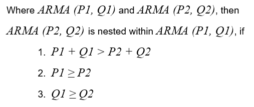
When beginning to look at using more complex ARMA models, lower order models may not always be nested within higher order ones. In order to determine whether a model is nested within another, we use the following definition:
For ARMA models we use a different approach to help determine the most suitable model. We first ensure we accept only those iterations where all coefficients are significant. We can then compare models by:
using an LLR test if the models in question are nested; or
comparing their resulting log-likelihood and information criteria values if models in question are not nested.
Log-likelihood measures the goodness of fit of a statistical model to a sample of data. The greater the likelihood the better the model ‘fits’ the data. However, a very high log-likelihood value will result in an ‘overfitted’ model which may then significantly underperform on unseen data.
To help counterbalance this effect, we can use penalising parameters to ensure the resulting model leads to a better fit. There are a variety of methods and assumptions used to calculate these parameters, all with varying degrees of accuracy and complexity. The most commonly used method is the Akaike Information Criterion (AIC), where the penalising parameter is simply a measure of the total number of parameters. The higher the number of parameters, the higher the penalty.
The AIC is an estimate for the quality of a model relative to another model. It can be used to determine which one of multiple models is most likely to be the best one for a given dataset. AIC scores are only useful when comparing against other AIC scores for the same dataset. A lower AIC score is better. AIC is calculated using the following formula:
AIC provides a relatively simple and quick measure for the quality of models and generally performs well especially for larger datasets. However, due to AIC only measuring the relative quality of models, there is a risk that all the tested models may actually fit poorly.
A variety of other measures have been developed such as, Bayesian Information Criteria (BIC), Deviance Information Criterion (DIC), Hannan-Quinn Information Criterion (HQIC) and Watanabe-Akaike Information Criterion (WAIC). Each varies in their application and may be something we explore in the future.
For now, we will continue using the AIC to measure model quality and to continue exploring the effectiveness of statistical models to help predict DMA flows.


