In 2022 we launched our Paradigm club project along with four UK water companies who were the pioneering members. As part of the first year of the project SME Water derived and rolled out version 1 of the Paradigm model, largely using data that was provided by the member clients. Version 1 was delivered through trials with each club member throughout 2023, allowing for the model to be tested and for Paradigm to be embedded within existing teams and processes. A key strength of the Paradigm delivery plan has been that through collaboration and data sharing between members, the model can be improved and honed across the three years of the project. By October 2023 the Paradigm club project entered its second year and we at SME Water were tasked with delivering model improvements that had been put forward during our initial client trials and technical lead sessions. These sessions have been invaluable in allowing our club project members to feed back and help prioritise the development stages of Paradigm, as well as allowing us at SME Water to present development plans and insights throughout the project.
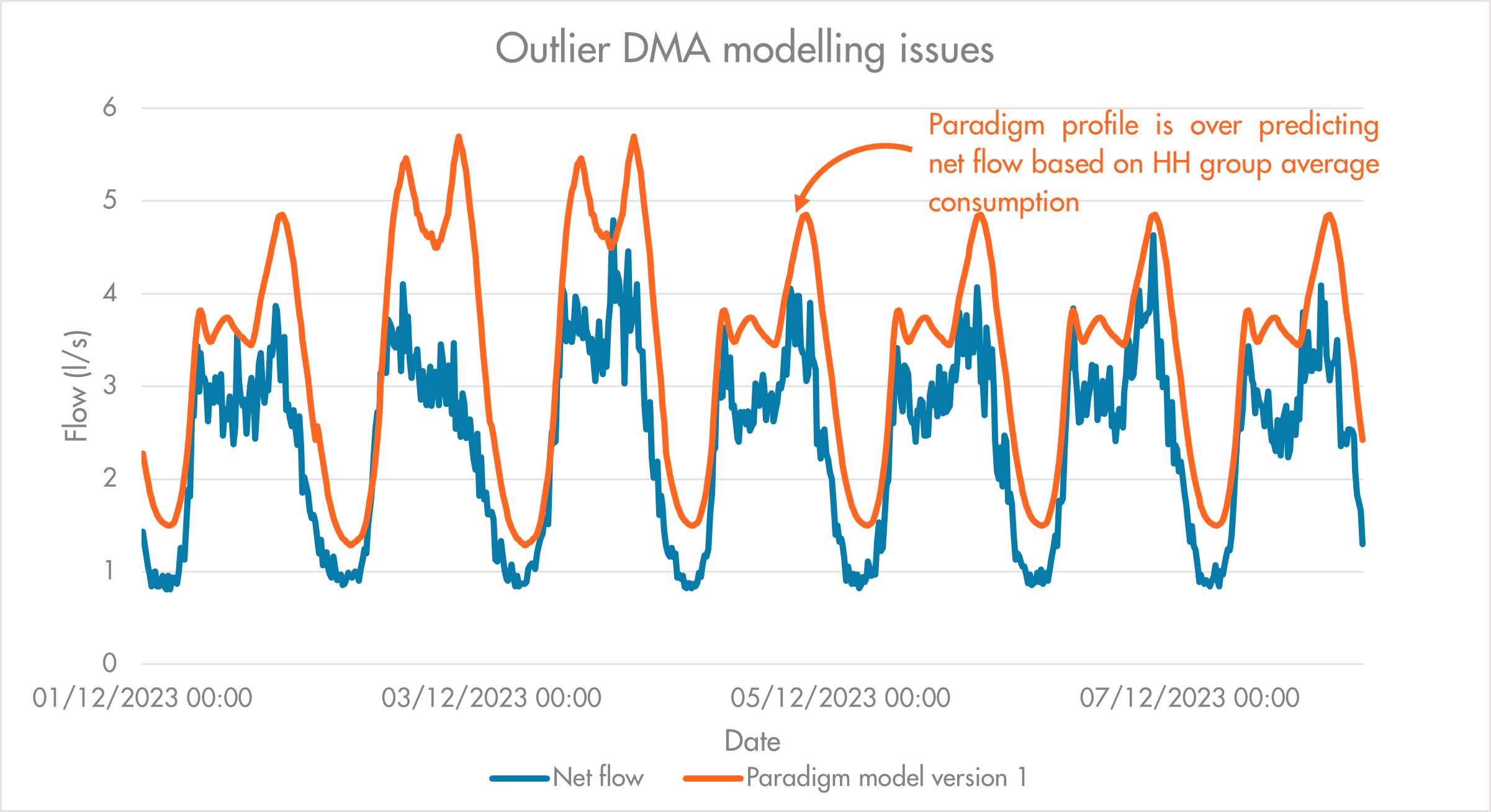
One of the key areas identified for model improvement was the household component of Paradigm. Whilst for the most part this component has worked well in version 1, there have been clear outliers that have caused issues when attempting to model DMAs with a more complex makeup; for example, higher than average occupancy or consumption values that have been proven to be lower than the expected model (figure i.).
Figure i. Modelling issues caused by unexpected DMA behaviour.
The cornerstone of the household component version 1 was the use client categorised household groups. Most UK water companies use Acorn data provided by CACI and recategorise this data based on household types within a DMA, and we received a conversion of this data to feed the household component in Paradigm. However, as Paradigm develops and our client base expands, we need the household component to be as flexible as possible to accommodate for the variability of water consumption, not only geographically but over time as well. This blog will give an overview of how version 1 uses this data and explore new datasets and techniques that are being used to improve how Paradigm models household consumption.
The Acorn data that CACI provides is primarily targeted at the retail and consumer sectors, helping to understand customer behaviour and demand for products in specific locations. Acorn data consists of seven key categories that group residents primarily by affluence, ranging from ‘Luxury Lifestyles’ to ‘Not Private Households’, with these categories comprising of subgroups and types to help better identify the demographics of households in an area. Water companies typically use this data to create their own groupings of households, and it was using this data that we created the initial household groups used in version 1. Each of our groups contained average consumption patterns, with each group being assigned a shape and associated volume that was aggregated up to DMA based on numbers of properties.
As our client’s household data is already categorised using a plethora of sources, utilising it can make it difficult to model an accurate representation of how water consumption will be used. All we are presented with is a household group and the count of each type within a DMA; this gives us no further information on key aspects that can affect consumption patterns such as occupancy, age, number of bathrooms etc. As we have no visibility of the individual variables within each group or how they have been grouped, we run the risk of modelling based on assumptions which increases the potential for error, especially as we aggregate the household component up to a DMA level.
A key limitation of Acorn data is that it is not open source and not all UK water companies have access to the data. This stops us from going back to the original Acorn data set and would reduce the potential pool of clients that could join the Paradigm club project if we did so, further highlighting the need to explore other data.
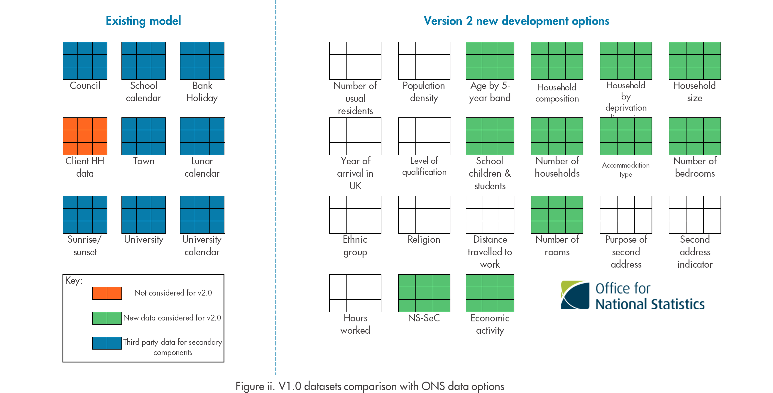
We were fortunate that as we began exploring alternative data to build version 2 of the household component, the Office of National Statistics (ONS) published the final release of 2021 census data. This has meant that we are able to access relatively recent data for all postcodes in England and Wales, with far greater granularity on households, residents and behaviours that can signpost changes in water consumption. Figure ii. shows the comparison in datasets available in version 1 (Existing model) and as part of version 2 development, including other third-party data that will be used to direct the secondary household components. But with this great expansion in data availability came a new problem…. How do we know which census data outputs affect customer water consumption?
Firstly, to improve the flexibility of the household component we decided that the shape and volume profiles needed to be separated in version 2. By removing the dependence on the group shape, we knew that the household volumes could more accurately represent what was happening in a given DMA, and we were confident that the newly acquired ONS data would provide enough detail to understand what variables caused changes in the volume of consumption.
To help winnow down this wide range of data we have been using Exploratory Factor Analysis to help identify which variables are related (correlate) to each other. This allows us to create groups of variables that show strong correlation and keep them separate from those they do not correlate well with. By doing this we create ‘Factors’; these can be described as the underlying or ‘hidden’ aspect that affects the variables within a group. There will usually be several factors possible within a group of variables, but by using Principal Component Analysis (PCA) we can see how well each variable correlates with the others, to make sure that only those with strong relationships are attributed to a factor. If you are unfamiliar with Factor Analysis and PCA then follow this link for an excellent summarisation of these techniques (https://youtu.be/Ollp2nSQCLY).
Choosing how many factors are pertinent to our data depends on how many of them are required to explain most of the original data’s variability. Purely looking at the data created by a PCA calculation does not give a conclusive answer, so we use two criteria to check where the cut off point should be. As the proportion of explained variability grows with each added factor, we eventually get diminished returns that make using extra factors less beneficial. Of course, using all possible factors would give us a 100% accurate model, but this would be extremely inefficient, so we settle for the majority of variability being explained by as few factors as possible.
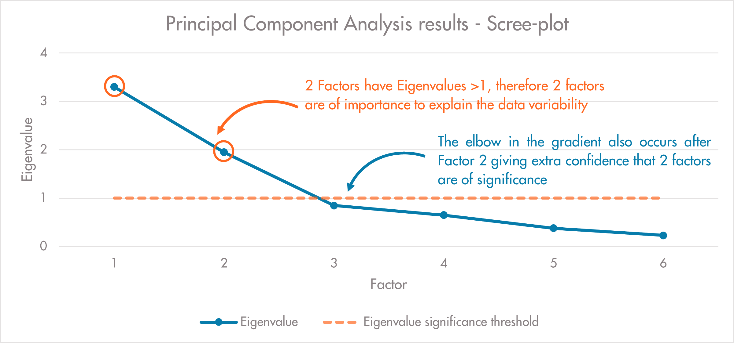
Figure iii. Eigenvalue criterion and scree-plot test example
To give a definitive answer of how many factors should be used, the most common tests are the Eigenvalue criterion and Scree-plot testing. At this point my mathematical brain starts to tune out, but simply put the eigenvalues denote the importance a factor has on the original data, the bigger the eigenvalue, the more likely we are to need this factor to explain the data’s variability. When plotted with Factors on the x-axis and Eigenvalue on the y-axis, the greater the eigenvalue, then the more importance this factor has on the variability of the dataset (Figure iii.). We take any eigenvalue above 1 as being significant in this test, so any factors with an eigenvalue >1 will be selected.
Scree-plot testing relies on the plotted data in figure iii. having a discernible elbow or ‘kink’ where the gradient of eigenvalue importance begins to plateau. Where this elbow begins to plateau shows where the factors being considered have reducing impact on the variability of the data, and so we take all factors to the left of the elbow as important enough to explain the majority of data variance. The example in figure iii. gives a simplified output where both the eigenvalue and gradient change occur after Factor 2, so we can be confident that it is these factors that account for the majority of data variance.
Within the ONS data, the results of these tests also showed two key factors that had a significant impact on volumetric consumption: household occupancy and affluence. These underlying factors affect several datasets from the census data but by normalising the variables and giving them a weighted score, we have been able to create two constants that can be applied to any DMA. These are then aggregated by number of household properties to give a volume we will use within version 2 of the household component.
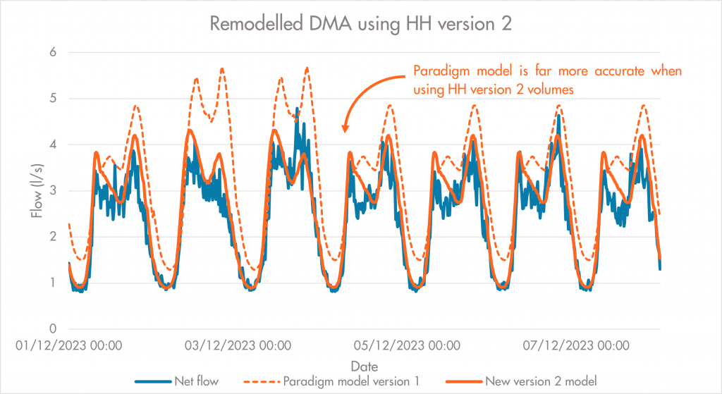
Figure iv. Modelling improvement made using HH version 2.
This method will hopefully provide the necessary flexibility to account for different behaviours in customer water consumption across our club project members’ DMAs. By separating the volume and shape profiles in version 2 of the household component we will not be limiting Paradigm’s ability to model those DMAs that do not conform to an average consumption in a particular demographic; any shape group can be given a totally unique volume based on the average occupancy and affluence, irrespective of demand patterns throughout the day or week (figure iv.).
Our next investigation currently in development is to utilise clustering and classification techniques to derive a more accurate group of household shapes using the ONS data, with initial shape improvements also visible in Figure iv. Following this, we will be analysing which demographic groups demonstrate strong seasonal trends that we can build into the household model, again increasing Paradigm’s flexibility and robustness to changes in water consumption.