Once per year at SME Water we each take on an ‘Assignment’. This is a self-selected research project undertaken in our learning and development time to further our skills in an area of interest. In this blog, I’ll share some of what I’ve learned this year about optimisation algorithms by applying them to help solve a problem with real relevance for leakage management.
Optimising Acoustic Logger Deployment with Genetic Algorithms
Introduction
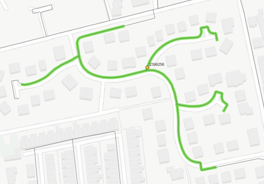
Figure 1 – Network coverage trace for one acoustic logger
In my previous blog, I wrote about my work on calculating the effective network coverage of acoustic noise logging. This used spatial analysis to ‘trace’ the distance each sensor could hear along adjacent mains based on their material type. Seeing this technique demonstrated, one client asked if it might also be used to help automate the tedious process of logger deployment planning. Mulling this over later, I realised that it was a great opportunity to further my programming skills by tackling an interesting optimisation problem and decided to give it a go.
Stay tuned to hear about the challenges I encountered, what I learned along the way and how I was ultimately able to achieve near-full DMA coverage using one third less loggers.
The Problem
Acoustic noise loggers (specifically accelerometer type) attach magnetically to existing fittings on the network. Which locations should they be deployed to? The results of my earlier effective coverage analysis highlighted that some areas of the network have a level of redundancy in their current acoustic logging, where the coverage of two adjacent loggers overlaps. At a basic level, this should be avoided to reduce hardware and maintenance costs. In other words, it would be desirable to achieve the same level of network coverage by using fewer loggers. Thinking about planning deployment for a new area of the network, we would like to both:
- Maximise network coverage, to give the highest chance that a burst will be detected by one of our sensors
- Minimise overlap between the coverage of adjacent loggers, so that we can save money by deploying and maintaining fewer loggers (while maintaining high effective coverage)
There are some further real-world considerations which could complicate things, but I decided to focus on this relatively simple optimisation as a learning exercise.
Approach
The aims & objectives of my assignment can be summarised as follows:
- Investigate how logger deployment planning might be automated, identifying techniques & algorithms which might be helpful
- Create a proof-of-concept solution which attempts to optimise deployment in a single DMA, to help explore the problem
I selected a DMA for testing based on it having a high fitting concentration on metallic mains (i.e., lots of potential overlap to resolve), and also some areas of plastic mains (Figure 2). There are 265 fittings which might be logged to help detect bursts on mains within this DMA. The goal is to decide which fittings to log or not. For a set of fittings, we can use the spatial analysis tools already developed to evaluate the mains length covered, and the number of loggers used.
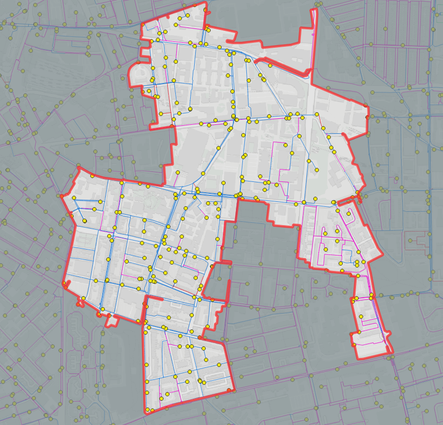
Figure 2 – Example DMA chosen for study
I pre-calculated the maximum achievable coverage in terms of metres of mains length by evaluating the result of logging all 265 fittings. For the chosen DMA, this would be around 22km out of 31km total mains length. A useful metric to help evaluate the quality of a candidate solution would be a coverage deficit, defined as the difference between this maximum achievable coverage and coverage of the chosen loggers.
Why not calculate all possible logging combinations and pick the best result? Well, as we have 265 Boolean choices to make, the number of possible combinations of logged fittings is 2265. This approximately the same as the number of atoms in our universe! We’re unlikely to ever have a computer big or fast enough to try 5.9×1079 ideas, which highlights the need for both an algorithmic approach, and to use our knowledge of the problem to reduce the size of the search space.
‘Critical’ fittings and the ‘compass’ approach
One way the problem can be made easier is by realising that some fittings are more important than others. There are some points which have zero (or near-zero) overlap with the coverage of other sensors. These should be logged, as we want maximum coverage and there is no conflict with potentially overlapping loggers which would need to be resolved.
This technique identified 54 critical fittings, which is a good start. But having only gained 15% of the achievable mains coverage, we have a long way to go!
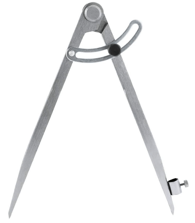
Figure 3 – The ‘compass’ approach
How else can knowledge of the problem domain be applied to help find a solution? Humans tend to approach deployment planning with what I like to call the ‘compass’ method. If a logger can hear 100m in both directions (e.g., metallic main), we can imagine using a compass set to 200m to walk along the pipe, repeatedly selecting the nearest fitting. This makes a lot of sense for a single, straight main with a lot of fittings, but DMAs are usually more complicated. Doing this manually can be time-consuming and confusing due to unclear connectivity and various mains materials – not to mention boring! Boredom will inevitably lead to carelessness and mistakes. All more the reason to develop an automated solution then.
The ‘compass’ method provided some inspiration, but I couldn’t quite get my head around what it should do in non-trivial situations encountered in real DMAs. Hesitant to just start coding and see what happens, at this point I decided to hit the books and do some research on more general approaches applicable to similar problems. This seemed like the right decision from a learning & development perspective, as the techniques learned from such an approach should be more transferable and useful in the future.
Genetic Algorithms
Still facing the problem of how to find good solutions among almost uncountable possibilities, I came across a book collecting dust in the office. The first few pages mentioned “many computational problems require searching through a huge number of possibilities for solutions,” explaining how “candidate solutions are encoded as strings of symbols” and that “a genetic algorithm is a method for searching […] for highly fit strings.” (Mitchell, 1998)
This timely coincidence caught my attention, so I decided to learn more and have a go at applying genetic algorithms to the problem at hand.
Genetic Algorithms (GA) are so-called because they attempt to emulate some concepts from biology, with the objective being to ‘evolve’ towards a strong solution. One fundamental concept is that a candidate solution is encoded as a chromosome. A chromosome is a string of symbols or bits representing the solution. In our example, let’s imagine that we have a simple area with only ten fittings – each of which we may or may not log. We can represent these choices with a string of ten bits, e.g., 0111011000.
GAs simulate reproduction and “survival of the fittest”, so they need a way to evaluate the fitness of an individual candidate solution. This is called the fitness function, and the algorithm will try to minimise it i.e., identify a solution for which this function returns the lowest possible value. In our case this should get higher (worse fitness) when:
- More loggers are used (encourage using less loggers)
- Coverage is less than the maximum achievable coverage
In a nutshell, genetic algorithms work by evaluating the ‘fitness’ of an initial population of candidate solutions and then having these ‘reproduce’, with their probability of selection increasing with better fitness. Over successive generations, the overall fitness of the population increases and hopefully produces some highly fit candidates, in a process which emulates biological evolution.
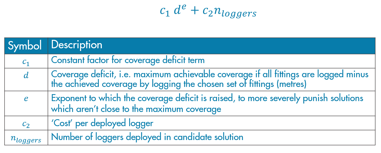
Figure 4 – Fitness function form with description of terms
After some initial experimentation, I settled on a form for my fitness function as shown in Figure 3. Here, the second term is simply the number of loggers multiplied by a cost per logger. The first term takes the coverage deficit and raises it to an exponent (greater than 1), to more severely punish solutions which are further away from the maximum achievable coverage.
The balance between these two additive terms determines how much the optimisation will prioritise coverage versus cost. Having established this, there then followed a period of experimentation with the values of the constants and exponents, and the parameters controlling the genetic algorithm run to learn more and try to produce the best possible result. I will spare you the details of this and summarise.
Using a population size of 100 candidate chromosomes per generation, I was initially running for 100 generations but noticed that sometimes the evolution had not yet plateaued. This indicated that continuing the runt o later generations might yield further improvement, so I began running the experiments all the way to 400 generations. As expected, the solutions continued to improve, and I was able to learn more about how I should tweak the fitness function.
Results
Figure 5 shows how the best solution from each generation continued to improve (lower minimised value) through the 400 generations simulated. The y-axis here shows the lowest (best) value fitness in each generation, calculated based on the formula shown in Figure 4 to give a single metric to evaluate how good a solution is. So what does this translate to in terms of our objectives of maximising coverage while minimising number of loggers deployed?
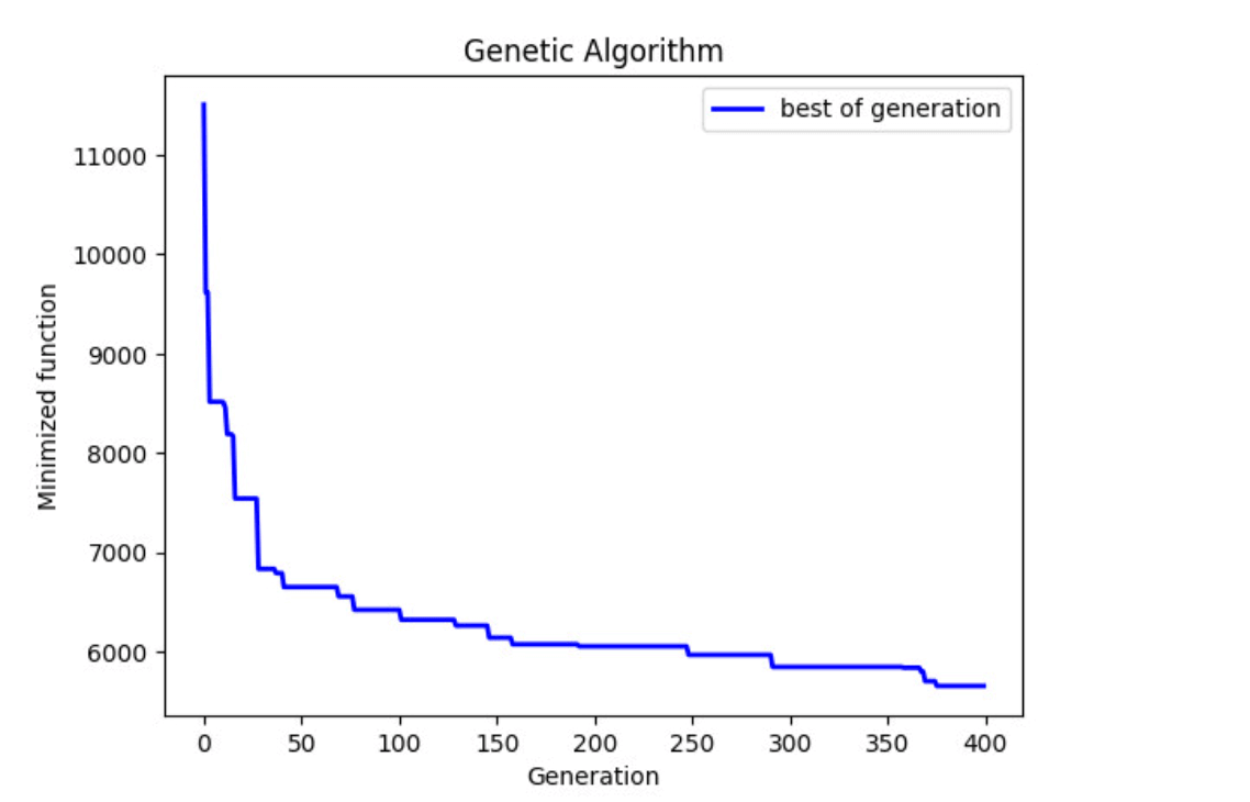
Figure 5 – Evolution of best candidate solution over 400 generations
The best solution found has a coverage deficit of less than 3.5% below the maximum achievable coverage with 91 fewer loggers deployed – a saving of more than a third on capital and operational expenditure. By this measure one could say that the assignment objectives have been met, and my experiments have proved the concept of using an algorithmic approach to optimise acoustic logger deployment planning.
Reflections
Because we don’t know what the optimum solution is, it’s hard to quantify how good a job the algorithm did. It would be useful to compare the solution to a human effort (and the time taken).
In terms of applying such analysis to a real deployment there are some further considerations. Some potential logging sites may have poor communications. If this was surveyed in advance then an additional term giving a penalty for low comms score might be added into the fitness function to allow the optimisation to consider this. It may not be possible to log some sites due to parked cars, seized covers or other unforeseen access issues. This raises questions about how the optimised results might be used in practice, where the unavailability of some fittings might require adapting the deployment plan to achieve near-optimal coverage.
I was only able to scratch the surface of this topic in the few days of effort available for my assignment project. Genetic algorithms are one of many possible approaches to this type of problem, and other interesting methods (e.g., Tabu search) remain unexplored. That said, these early results show the clear potential to find efficiencies at the deployment planning stage which will continue to provide the benefit of reduced operational costs throughout the lifespan of the fleet.
It was good to gain some experience in this area and continue adding to my ‘toolbox’ of analysis techniques. I look forward to more opportunities to innovate and work on similarly interesting problems in the future.