DMA demand analysis is an integral part of a leakage analyst’s job. Being able to confidently determine whether a sustained increase in night usage within a DMA is due to a rise in leakage or due to an increase in customer consumption is vital. We are currently amidst Ramadan, the time of the year that leads to no end of confusion. In most cases, leakage teams simply suspend leakage targeting in DMAs affected by Ramadan. In some DMAs, the nightline simply returns to normal after Ramadan, but in many other areas, the nightline remains high. How can we explain this? Is this due to some other unexplained consumption, or is this due to leakage? It is difficult to take action with so much uncertainty, so how do we tackle this problem?
Enter Paradigm, our DMA demand forecasting model. Paradigm is different from other time series forecasting models because it doesn’t just forecast solely based on historical analysis. Instead, it builds its forecast from a DMA’s attributes and customer information. Therefore, it assists in understanding ‘what should my DMA be consuming?’, as well as ‘what will my DMA be consuming?’. We have found this approach for modelling DMA consumption to be highly effective in identifying DMA anomalies.
Residual analysis
So how does Paradigm help to identify DMA anomalies? There are many ways to determine the statistical accuracy of a forecasting model. One of them is to conduct residual analysis, where the residuals of a model are simply the difference between the actual (observed) and predicted (expected) values. The general idea is that the smaller the residuals, the more accurate the model. This concept is expanded for a time series forecasting model and an accurate time series forecast is where the residuals exhibit the properties of ‘white noise’.
White noise accounts for the natural error in a sample which is unavoidable. Analysing the residuals for each DMA for each day and checking how close to white noise each forecast is gives us an excellent method to determine how accurate our model is. If our model is accurate, then so is our understanding of the DMA. Where the residual from a forecast does not result in white noise, we can analyse the shape of the residual profile to infer useful insights into the shortcomings of our model. The following examples help explain and expand on this idea.
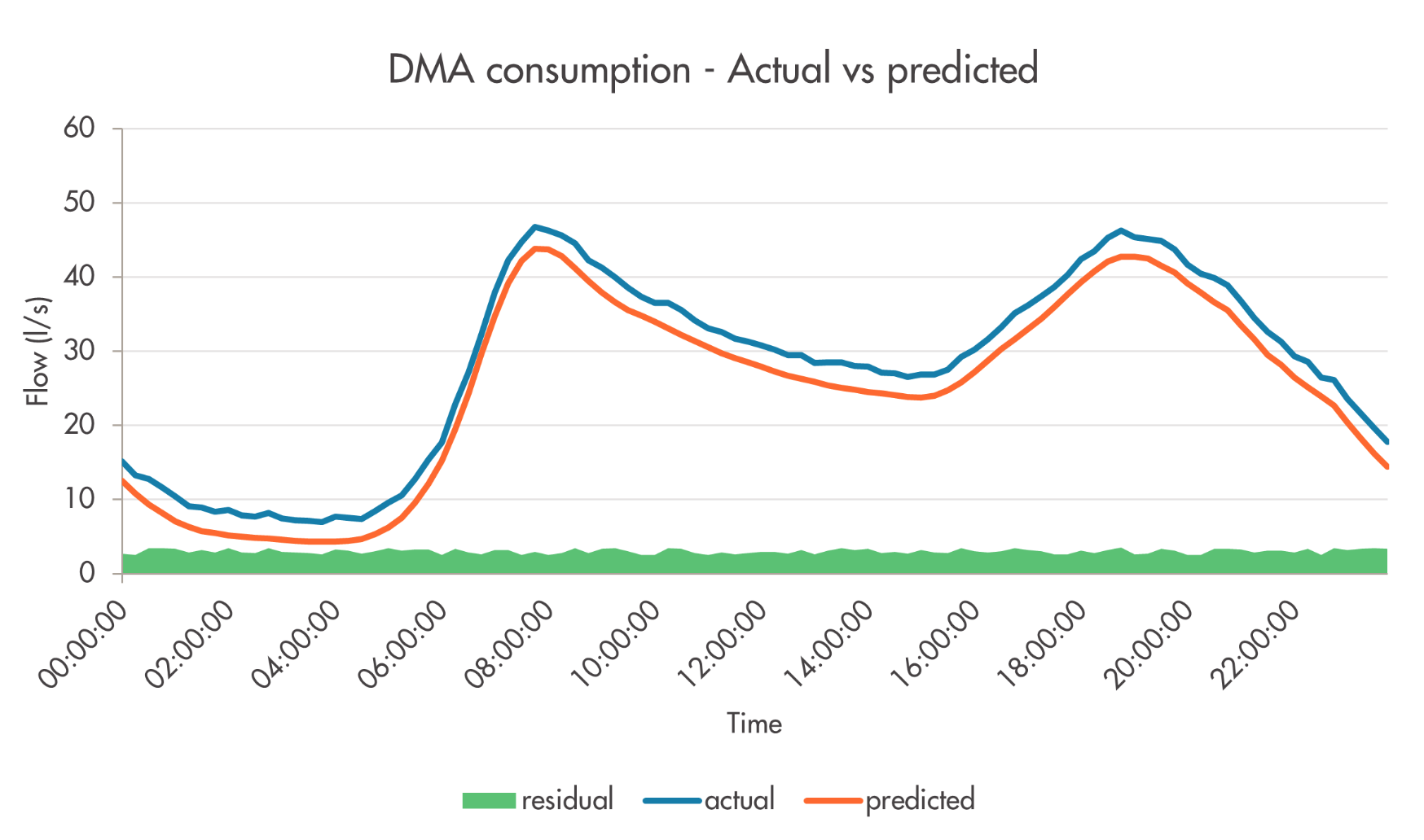
Example 1 – Prediction with a flat profiled residual
Figure 1: Example of a DMA prediction with a flat profiled residual
In this example, the difference between the actual and predicted DMA consumption returns a flat profile. This implies that there is a continuous unaccounted for flow, which can be explained by a burst (network or customer) or by unknown customer usage. After this, localisation techniques or property-level analysis can be carried out to help identify the issue within the DMA.
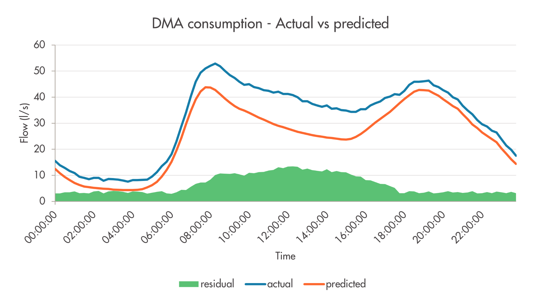
Example 2 – Prediction with a NHH-shaped residual
Figure 2: Example of a DMA prediction with a NHH-shaped residual
In this example, the difference between the actual and predicted DMA consumption returns a profile with increased consumption during working hours. This tends to imply that there is unknown non-household usage. There is a clear difference between weekday and weekend residuals in some cases, where some DMAs have very little unaccounted for water during the weekend (and therefore have an accurate prediction) but vary significantly during the weekday. Observing the change in this unaccounted for water throughout the year helps us begin to understand the varying consumption of non-households, which we can then use to improve our forecast going forward.
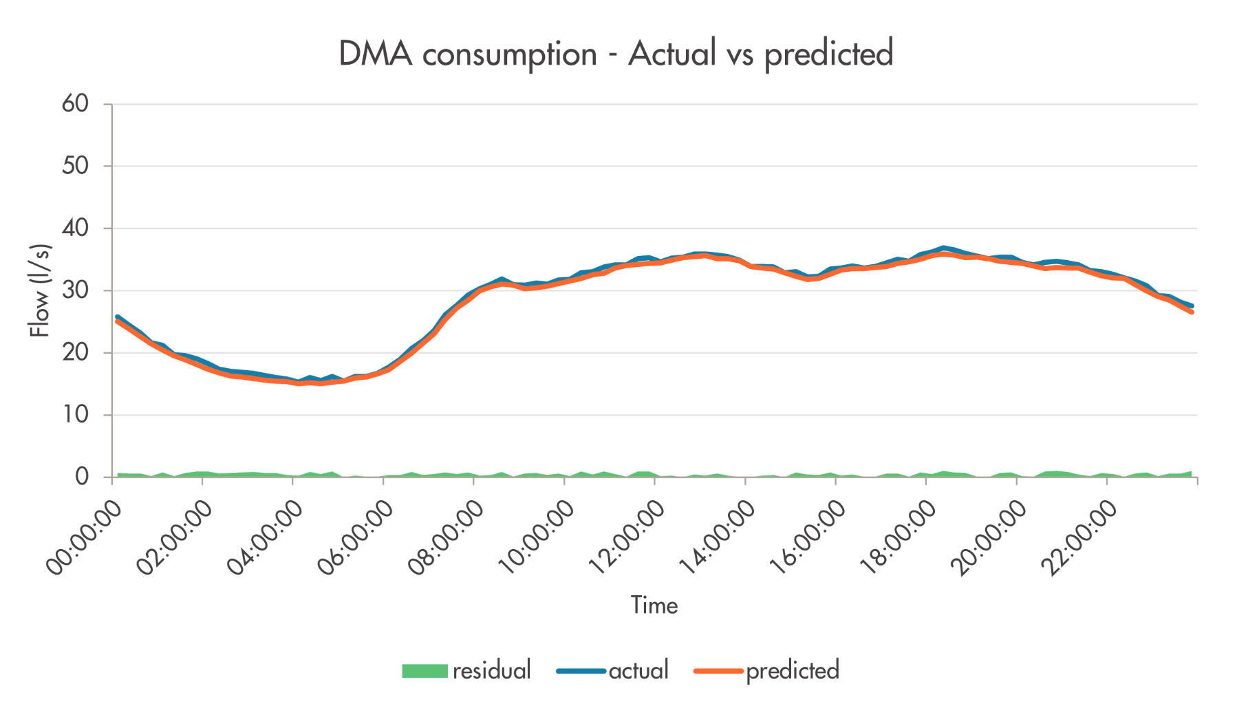
Example 3 – Prediction in an area with high occupancy
Figure 3: Example of a DMA prediction in an area with high occupancy
In this example, the difference between the actual and predicted DMA consumption returns a ‘white noise’ profile. This implies that the prediction is accurate. This example is especially interesting because a leakage analyst might look at this diurnal profile and conclude that this DMA has a higher-than-expected nightline and must therefore have leakage. This is because a leakage analyst would be looking for a ‘typical’ DMA profile, as shown in the previous examples. Paradigm differentiates between various household groups based on their Acorn (consumer classification) type, and in the example above, the predicted diurnal profile is typical of high occupancy households. This allows the leakage analyst to confidently determine that the previously unknown night flow is, in fact, domestic consumption and not leakage.
Conclusion
The three examples provided here begin to show how we can use residual analysis to identify anomalies or unaccounted for water within DMAs with some degree of confidence. There are many other insights that can be gained from analysing residuals, including identifying DMA boundary changes, identifying new housing developments, and determining seasonal usage. These examples provide plenty of opportunities to continue improving the predictions generated by Paradigm.